Your name: Jerry Liu
Your UID: 404474229
Please upload only this notebook to CCLE by the deadline.
Policy for late submission of solutions: We will use Paul Eggert's Late Policy: $N$ days late $\Leftrightarrow$ $2^N$ points deducted} The number of days late is $N=0$ for the first 24 hrs, $N=1$ for the next 24 hrs, etc., and if you submit an assignment $H$ hours late, $2^{\lfloor H/24\rfloor}$ points are deducted.
NOTE: In this assignment we provide pseudocode to get you started.
In later assignments we will not do this.
Problem 1: SVD k-th order approximations (30 points)
If $A$ is a matrix that has SVD $A = U\,S\,V'$, the rank-k approximation of $A$ keeping only the first $k$ columns of the SVD.
Specifically, given a $n \times p$ matrix $A$ with SVD $A = U\,S\,V'$, then if $k \leq n$ and $k \leq p$, the rank-$k$ approximation of $A$ is $$ A^{(k)} ~~=~~ U ~ S^{(k)} ~ V' $$ where $S^{(k)}$ is the result of setting all diagonal elements to zero after the first $k$ entries $(1 \leq k \leq p)$. If $U^{(k)}$ and $V^{(k)}$ are like $U$ and $V$ but with all columns zero after the first $k$, then $$ A^{(k)} ~~=~~ U ~ S^{(k)} ~ V' ~~=~~ U^{(k)} ~ S^{(k)} ~ V^{(k)'} . $$
In class, we saw a demo of the attached Matlab script imagesvdgui.m --- and the effectiveness of this approximation in retaining information about an image.
The goal of this problem is to implement this approximation for black-and-white (grayscale) images.
load mandrill
Mandrill = ind2rgb(X, map);

A = mean( Mandrill, 3 );  % grayscale image -- size 480 x 500.
size(A)

imwrite(A, 'GrayMandrill.bmp')  % Write the Mandrill to a bitmap image file

% The matrix A now contains the Mandrill image (in grayscale)
Display the bitmap image file using an HTML img tag:
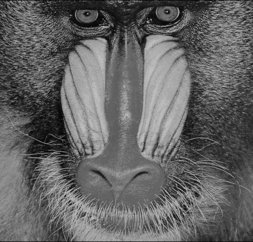
<img src="resources/GrayMandrill.bmp">
1.(a): Plot Singular Values of the Rank-$k$ Approximation of an Image
As in HW0, construct a grayscale version of the Mandrill image, and take one of the 3 color planes as a 500x480 matrix. This is our `black and white' image $A$. You are to analyze the rank-k approximation of the image.
Compute the SVD of $A$, and plot the singular values $\sigma_1$, $\sigma_2$, ...
[U S V] = svd(A);       % U, S, V are now the SVD of A

norm( A - U * S * V' )  %  A should match the product of U, S, V'

X = diag(S);
plot(X);

1.(b): Optimal Rank-$k$ Approximation of an Image
Find the value of $k$ that minimizes $\mid\mid{A \; - \; A^{(k)}}\mid\mid^2_{F} ~+~ k$.
[n p] = size(A);
[U S V] = svd(A);
maximum_possible_k = min(n,p);
min_err = max(n, p);
singular_vals = diag(S).^2;
minK = 0;

for k = 1 : maximum_possible_k
    err_sum = (sum(singular_vals((k + 1) : maximum_possible_k)) + k);
    if err_sum < min_err
        min_err = err_sum;
        minK = k;
    end
end
minK
1.(c): The Rank-$k$ Approximation is a Good Approximation
In the chapter on the SVD, the course reader presents a derivation for $A \, - \, A^{(k)}$: $$\begin{eqnarray*} A \; - \; A^{(k)} & = & U \; S \; V' ~ - ~ U^{(k)} ~ S^{(k)} ~ V^{(k)'} \\ & = & U \; S \; V' ~ - ~ U \; S^{(k)} \; V' \\ & = & U \; (S ~ - ~ S^{(k)}) \; V ' \\ \end{eqnarray*}$$
Prove the following: $$ \mid\mid{A \; - \; A^{(k)}}\mid\mid^2_{F} ~=~ \sum_{i>k} \sigma_i^2 . $$
Proof (Enter your Proof here)
Because $A \; - \; A^{(k)} ~ = ~ U \; (S ~ - ~ S^{(k)}) \; V '$,
As a result, $\mid\mid{A \; - \; A^{(k)}}\mid\mid^2_{F} ~ = ~ \text{tr}((U(S - S^{(k)})V')(U(S - S^{(k)})V')') = \text{tr}((U(S - S^{(k)})V')(U^{-1}(S - S^{(k)})'(V')^{-1})) $
$= \text{tr}(UU^{-1}(S - S^{(k)})(S - S^{(k)})'V'(V')^{-1}) = \text{tr}((S - S^{(k)})(S - S^{(k)})') = \sum_{i > k} \sigma_i^2$
Therefore $$ \mid\mid{A \; - \; A^{(k)}}\mid\mid^2_{F} ~=~ \sum_{i>k} \sigma_i^2 . $$
Problem 2: Baseball Visualization (40 points)
For this dataset you are given a matrix of statistics for Baseball players. You are to perform two kinds of analysis on this matrix.
Read in the Baseball Statistics
Statistics of top players after the last regular season game, obtained from MLB.com, October 2016.
%%% Stats = csvread('Baseball_Players_Stats_2016.csv', 1, 0);  # skip the header (= row 0)
%%% Names = csvread('Baseball_Players_Names_2016.csv', 1, 0);

Baseball_Players_2016   %% execute Baseball_Players_2016.m  to load in the data needed here
StatNames{1:3}

size(StatNames)

StatNames{:}
size(Stats)
Stats(1:3, :)
size(PlayerNames)
PlayerNames{1:3}
Compute a "scaled" version of the Stats matrix
We scale each column of values ${\bf x}$ in Stats to be ${\bf z} = ({\bf x}-\mu)/\sigma$ in ScaledStats, where $\mu$ is the mean of the ${\bf x}$ values, and $\sigma$ is their standard deviation.
In Octave/Matlab, the function mean() computes column means, and std() computes standard deviations. The function zscore() computes both, and uses them to "scale" each column in this way.
This scaling is also called normalization and standardization. The z-scores ${\bf z} = ({\bf x}-\mu)/\sigma$ are also called the standardized or normalized values for ${\bf x}$.
ScaledStats  =  zscore(Stats);   %  z  =  (x-mu)/sigma

mean(ScaledStats)  %  the means of each column after normalization should be 0
std(ScaledStats)   %  the standard deviations of each column after normalization should be 1
2 (a): Random Projections
A fundamental problem in data science is that it is impossible to visualize a dataset that has many features. Given an $n \times p$ dataset (matrix) $A$ in which the number of features $p$ is large, there is no obvious way to plot the data.
Dimensionality reduction algorithms have been developed that attempt to find datasets that have lower values of $p$ but approximate $A$ in some way. Although there are sophisticated algorithms, a competitive approach is to compute a random projection of $A$ into a few dimensions. When the projection is into 2 or 3 dimensions, the result can be visualized.
A random $k$-D projection of a $n \times p$ dataset (matrix) $A$ is the result $(A \, P)$ of multiplying $A$ on the right by a $p \times k$ matrix $P$ of random values.
The result is a $n \times k$ matrix, assigning each row in $A$ a new pair of values $(x,y)$, and these can be interpreted as positions in a 2D plot.
% plotting 2D values
Iris = csvread('iris.csv', 1,0);  % skip over the header line
A = Iris(:, 1:4);  % just the measurement columns
[n p] = size(A);
P = rand(p,2);
disp('random projection weights:')
disp(P)
XY = A * P;
plot(XY(:,1), XY(:,2), 'b.')
title('random projection of the iris data')
species = {'  s', '  v', '  V'}
text(XY(:,1), XY(:,2), species(Iris(:,5)), 'FontSize', 10 )
Problem: write a function random_projection(A,k) that, given an input matrix $A$ of size $n \times p$ and an integer $k>0$, produces a random $k$-D projection.
Please use uniform random values in the matrix $P$.
Then: plot the result of 3 random 2D projections of the data.
In each plot, identify the greatest outlier -- the player with $(x,y)$ values that have the largest total $x+y$. Print the row in the dataset whose projection is this outlier.
random_projection = @(A,k) A * rand(size(A, 2), k); % fill in using e.g.:   ... rand(size(A,1),k) ...

for i = 1 : 3
    XY = random_projection( ScaledStats, 2 );
    subplot(3, 1, i);
    if i == 1
        xcolor = 'rx';
    elseif i == 2
        xcolor = 'bx';
    else
        xcolor = 'gx';
    end
    plot(XY(:,1), XY(:,2), xcolor)
    if i == 1
        title( 'Random 2D Projection of Scaled States Matrix' )
        legend('1st run', 'Location', 'northwest', 'Orientation', 'Horizontal');
    elseif i == 2
        legend('2nd run', 'Location', 'northwest', 'Orientation', 'Horizontal');
    else
        legend('3rd run', 'Location', 'northwest', 'Orientation', 'Horizontal');
    end

    XplusY = sum(XY, 2);
    [maxXplusY, greatest_outlier] = max(XplusY);
    fprintf('The outlier row for %d th run is row %d: \n', i, greatest_outlier);
    ScaledStats(greatest_outlier, :)
    names = strcat(PlayerNames(greatest_outlier), ', ');
    ranks = PlayerRanks(greatest_outlier);
    textStr = strcat(names, ranks);
    text( XY(greatest_outlier, 1), XY(greatest_outlier, 2), textStr, 'FontSize', 5 );
end

2 (b): Latent Semantic Analysis
The course reader describes Latent Semantic Indexing for a matrix of values measuring association between X terms vs. Y terms.
The classic example is a "term/document matrix" for Keywords vs. Books, shown below. The code shown produces an LSI plot for the data.
Your job is to produce an analogous LSI plot for the table of Baseball players.
Components are computed as in: Berry, M. W., Dumais, S. T., and O'Brien, G. W. (1995). "Using linear algebra for intelligent information retrieval." SIAM Review, 37(4), 1995, 573-595.
Some LSI references: lsi.research.telcordia.com/lsi/LSIpapers.html
nX = size(StatNames, 2)

% PlayerNames:  Stats Attr

nY = size(PlayerNames, 1)

% ScaledStats:
% Stats Attr: 1  2  3  4  5  6  7  8  9 10 11 12 13 14 15 16 17   % Players:
%--------------------------------------------------------------------------
% ScaledStats':
% Players: 1 2 3 4 ... 146 % Stats Attr:
%                             Rank
%                             G
%                             .
%                             .
%                             .

[U,S,V] = svd(ScaledStats');

%  We can look at a plot of the singular values (diagonal of S):

plot( diag(S), 'b' )

Xfactor = U(:,1:2);
Yfactor = V(:,1:2);

% plot the 2D projection of the data

text_offset = 0.01;
plot( Xfactor(:,1), Xfactor(:,2), 'r*' )
hold on
plot( Yfactor(:,1), Yfactor(:,2), 'b*' )

for i = (1:nX)
     text( Xfactor(i,1)+text_offset, Xfactor(i,2), StatNames(i), 'FontSize', 4)
end

for i = (1:nY)
     text( Yfactor(i,1)+text_offset, Yfactor(i,2), PlayerNames(i), 'FontSize', 4)
end

title( 'Latent Semantic Indexing:  Players vs. Stats Names' )
xlabel( '1st component' )
ylabel( '2nd component' )
axis([-0.3, 0.4, -0.45,0.38]);

zoom on
hold off

Problem 3: Global Warming again (30 points)
In HW0, you plotted the average (non-missing-value) temperature anomaly over the entire grid, for every year from 1916 to 2015.
In this problem we want you to fit linear models through the data.
% set up everything as in HW#0:

GHCN = csvread('ghcn.csv');

%   The data was artificially shifted to [0, 4500];
%     its range should be [-2500, +2000]/100 = [-25,+20], in degrees Centigrade.
%     Since our focus here is on warming, we ignore temperatures below -5.
%   We omit the year and month in columns 1:2 before scaling:

GHCN_in_centigrade  = (GHCN(:,3:74) - 2500) / 100;

temperature_anomaly = reshape( GHCN_in_centigrade, [36, 12, 137, 72] );   % convert to a 4D matrix, so we can use slices

missing_values = (temperature_anomaly == -25);
number_of_missing_values = sum(sum(sum(sum( missing_values ))));

maximum_anomaly_value = max(max(max(max( temperature_anomaly ))));
minimum_anomaly_value = min(min(min(min( temperature_anomaly .*  (~ missing_values) ))));  %  '~' is 'not' in MATLAB

US_latitude  = 9:12
US_longitude = 15:20
my_years = 1916:2015;
my_slice = temperature_anomaly( US_latitude, :, my_years - 1880 + 1, US_longitude );

total_number_of_grid_squares = length(US_latitude) * length(US_longitude) * 12;
N = total_number_of_grid_squares;

average_US_anomaly_by_year = reshape( sum(sum(sum( my_slice, 4),2),1), [length(my_years) 1] ) / N;

plot( my_years, average_US_anomaly_by_year )
xlabel('year')
ylabel('avg anomaly (Centigrade) in the US')
title('average US temperature anomaly by year')

(a) Global Average Temperature Anomaly: Linear Model (Least Squares)
Problem: fit a line through the data, using Least Squares.
my_years = 1916:2015;
temparature_nonmissing_anomaly = temperature_anomaly .*  (~ missing_values);
my_slice = temparature_nonmissing_anomaly( :, :, my_years - 1880 + 1, : );

total_number_of_grid_squares = 36 * 72 * 12;
N = total_number_of_grid_squares;

average_global_anomaly_by_year = reshape( sum(sum(sum( my_slice, 4),2),1), [length(my_years) 1] ) / N; % fill in something % ..........
nRows = size(my_years, 2);
my_years_A = [my_years', ones(nRows, 1)];

linear_model = my_years_A \ average_global_anomaly_by_year %  fit_curve( my_years, average_global_anomaly_by_year )  % ..........

plot( my_years, average_global_anomaly_by_year );
hold on;
X = [linspace(1916, 2015, 10000)' ones(10000, 1)];
Y = X * linear_model;
plot(X, Y);
axis([1900,2020,-0.3,0.2]);
xlabel('year')
ylabel('avg global anomaly (Centigrade)')
title('average global temperature anomaly by year')

(b) Global Average Temperature Anomaly: Piecewise Linear Model (Least Squares)
Problem: fit a 2-segment piecewise linear model through the data, using Least Squares.
Specifically, find a pair of least squares models, one from 1916 up to year Y, and one from year Y+1 to 2015, such that the SSE (sum of squared errors) is minimized.
minimum_SSE = max(average_global_anomaly_by_year) - min(average_global_anomaly_by_year);
linear_model_1 = ones(2, 1);
linear_model_2 = ones(2, 1);
YSelected = 1917;

for Y = 1917:2013
    year_up_to_Y = 1916 : Y;
    year_up_to_Y = [year_up_to_Y', ones(size(year_up_to_Y, 2), 1)];
    average_global_anomaly_by_year_up_to_Y = average_global_anomaly_by_year(1 : (Y - 1915));
    average_global_anomaly_by_year_after_Y = average_global_anomaly_by_year((Y - 1914) : 100);
    year_after_Y = (Y + 1) : 2015;
    year_after_Y = [year_after_Y', ones(size(year_after_Y, 2), 1)];
    linear_model_up_to_Y = year_up_to_Y \ average_global_anomaly_by_year_up_to_Y;
    linear_model_after_Y = year_after_Y \ average_global_anomaly_by_year_after_Y;
    Y_year_up_to_Y = year_up_to_Y * linear_model_up_to_Y;
    SSE_up_to_Y = (average_global_anomaly_by_year_up_to_Y - Y_year_up_to_Y)' * (average_global_anomaly_by_year_up_to_Y - Y_year_up_to_Y);
    Y_year_after_Y = year_after_Y * linear_model_after_Y;
    SSE_after_Y = (average_global_anomaly_by_year_after_Y - Y_year_after_Y)' * (average_global_anomaly_by_year_after_Y - Y_year_after_Y);
    total_SSE = SSE_up_to_Y + SSE_after_Y;
    if (total_SSE < minimum_SSE)
        linear_model_1 = linear_model_up_to_Y;
        linear_model_2 = linear_model_after_Y;
        YSelected = Y;
        minimum_SSE = total_SSE;
    end
end
plot( my_years, average_global_anomaly_by_year );
hold on;
X_1 = [linspace(1916, YSelected, 10000)' ones(10000, 1)];
Y_1 = X_1 * linear_model_1;
plot(X_1, Y_1);
X_2 = [linspace(YSelected + 1, 2015, 10000)' ones(10000, 1)];
Y_2 = X_2 * linear_model_2;
plot(X_2, Y_2);
axis([1900,2020,-0.3,0.2]);
xlabel('year')
ylabel('avg global anomaly (Centigrade)')
title('average global temperature anomaly by year')
minimum_SSE
YSelected
linear_model_1
linear_model_2
